With the introduction of Large Language Models (LLMs) Google and Microsoft are in war to see who will emerge as the go-to digital knowledge destination, evolving the web search paradigm we’ve known for the past 30 years. LLM-based systems are quickly becoming a massive oracle, helping “organise the world’s information”. LLMs are allowing retrieving answers (information) to queries (questions) on vast corpuses of billions of structured data documents. World-scale information retrieval systems are hard to build, hard to scale, and hard to operate. Large knowledge systems based on LLMs, if we would call these the successors of traditional web search, leverage the system architectures used for decades to scale information retrieval to corpuses consisting of billions of documents and millions of queries.
Related posts:
We must look back for inspiration and learnings in web-scale search architectures, and generally multi-task information retrieval architectures. This document is a primer on how IR systems are built.
Overview
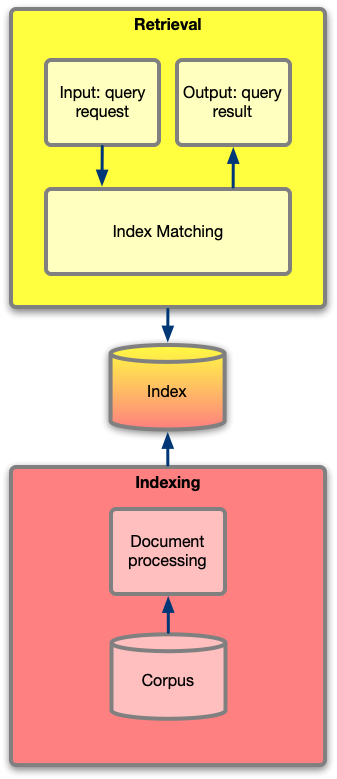
An information retrieval system consists of two core subsystems: indexing and retrieval.
- The indexing takes all input documents in the corpus to become part of the candidate results set and performs transformations, including preprocessing, analysis and indexing into a suitable stateful representation.
- The retrieval is responsible for performing all the necessary preprocessing, query analysis and augmentation, and post processing in order to go from query to result set. Finally the matching takes input queries that have gone through query management and finds the closest matching documents in the database. The retrieval is the interface that users interact with.
Retrieval
When we do a search query in Google or Bing, the query goes into a query management process to prepare it, then matching to generate a result set, and finally post processing of the result set. We’ll see each of these in more detail now.
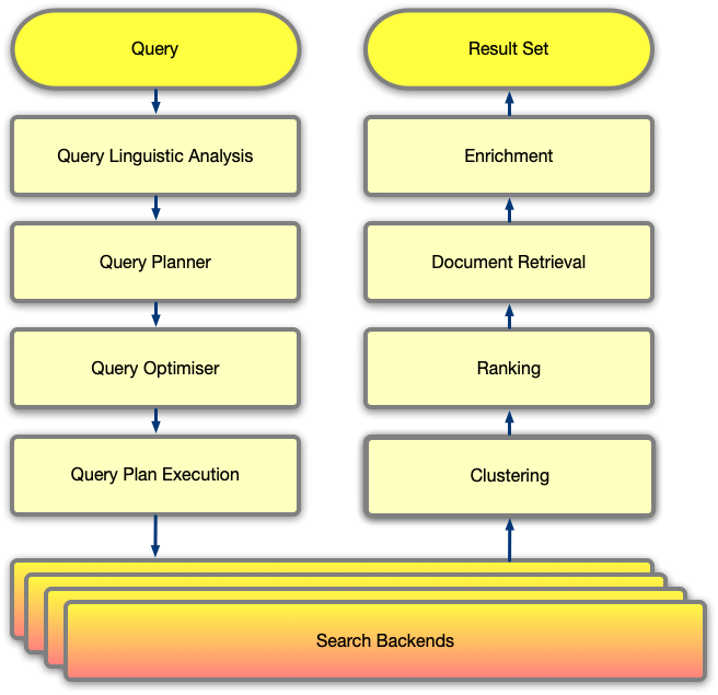
Query Management
- Query linguistic analysis (QLAS): the input query is broken down into a digital form which allows computers to reason about. In the current search systems, this phase consists of breaking down input sentences and keywords into “grams”. Grams could simply be words, or could be phonemes, letters, characters derived through stemming and tokenisation. The input query is transformed into “n-grams”, the sequence of n grams, meaning the 1-gram, 2-gram, 3-gram … 5-gram. The number of n-gram sequences to create depends on the complexity of the domain space and the available computation resources.
- Query planner (QP): once the n-grams are known, there is a mapping problem to decide which search backends to query, with what inputs, and what budget (time). The IR system has tens of different search backends, each optimised for a corpus and information domain, for example web pages, stocks quotes, images, news, etc. The greedy solution to any query is firing against all backends, yet this is wasteful, as for example a question about the latest attack in a war conflict would have the maximum information in the news backend, and probably very limited in the stock market quotes backend. The objective of the QP is to prioritise the queries that are about to be executed so that only the backends that will yield more information entropy, and select the n-grams that are more suitable for each backend. The QP also determines the order of execution of the queries, whether they should run sequentially or in parallel, and whether re-ranking of each result set is required.
- Query optimisation: backend loads will vary over time, as function of each corpus size and query volumes. The query optimiser ensures that the QP can be optimally executed given the current state of the system.
- Query plan execution (QES): Given an input QP, the QES is responsible for coordinating the execution across multiple search backends. QES transforms the input n-grams, queries backends, assigns time-budgets and handles timeouts, and merges or re-ranks results as required. The query “news about the latest attack from Ukraine is Moscow” could result in a query to the web search index with the raw terms and a budget of 300ms, another one to the knowledge base with the entities Ukraine and Moscow and a budget of 500ms, and another one to the news backend with 3, 4 an 5-grams with a budget of 800ms. The QES could then re-rank web search and news result sets, select the top 10 results, and finally merge the knowledge base result set on top. And the physical level, each search consists of many servers, structured as farms with columns (shards) and rows (replicas). Note that there might also additional execution strategies, such as demultiplexing & multiplexing network calls, in order to meet time budgets.
Matching & Result Management
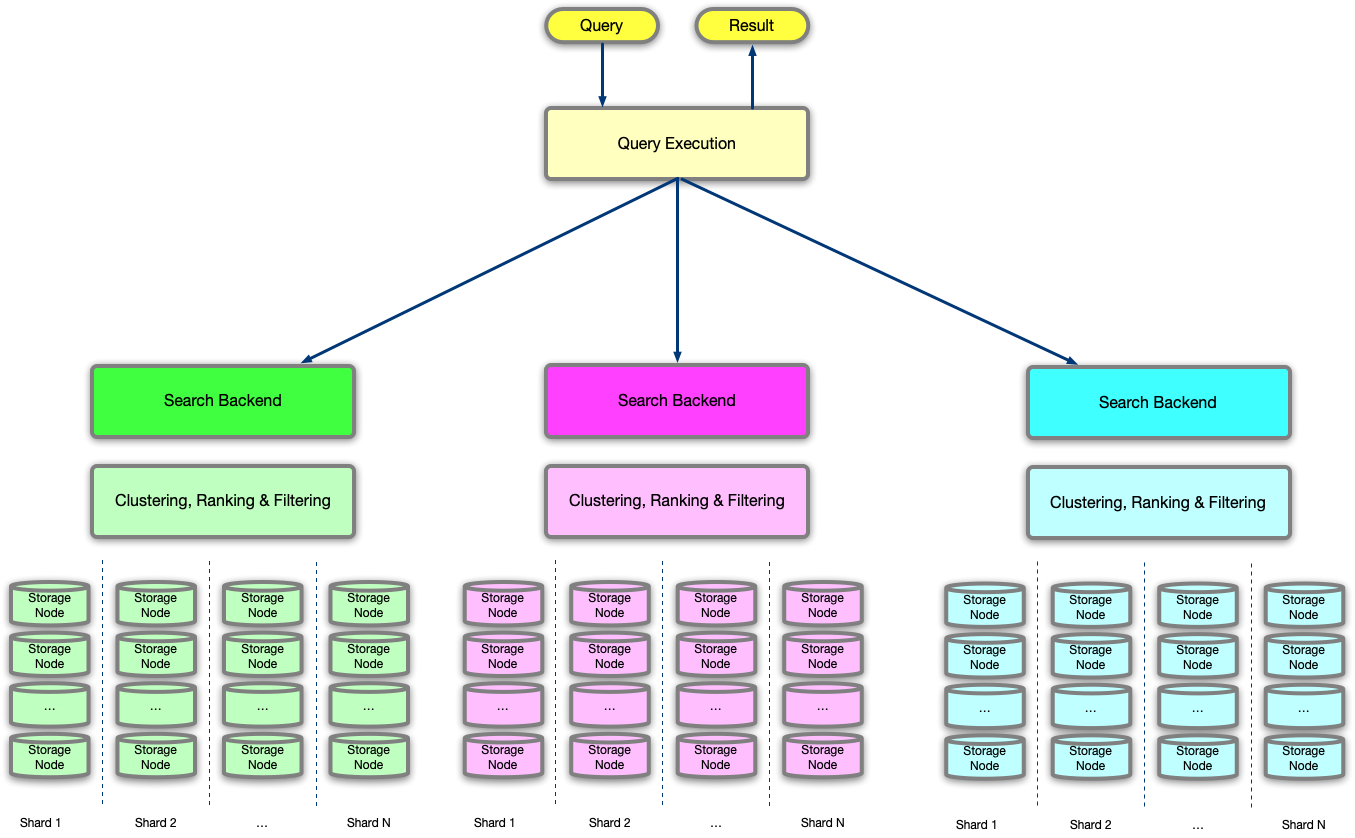
- Query execution (QE): the QE makes individual query requests to each search backend. The QE is a client of each search backend and responsible for managing the query timeout. The main complexity of the QE is maximising CPU, as qyery execution is a pure net-IO bound workload, with limited CPU computation occurring. This makes it a prime candidate for async IO serving using a reactor architectural pattern, force inbound network queuing, and avoid running out of client socket ports and file descriptors. The QE also acts as an intermediary proxy, and usually copying byte-by-byte response buffers from each search backened to QES, up to the timeout, when both up-stream and down-stream are closed.
- Search backend: each search backend is an homogeneous IR system for a particular task, domain, and/or query type. For example, the backend of the most popular web pages; or the backend of all Facebook web pages, or all news articles from today. There are a few types of possible search backends, the most common ones being:
- Boolean search, usually on a binary tree. These are expensive queries, and provide a deterministic result (probability = 100%).
- Relational query, usually on a B-tree. These are very expensive queries, and provide a deterministic result (probability = 100%).
- Term-based search, usually on an inverted index with posting lists. These are cheap queries, and provide a probabilistic result.
- Vector-based search, usually on an inverted index using weights. These are relatively cheap, but not as cheap as term-based queries, and provide a probabilistic result (cosine similarity being the most common option).
- Query ranking: search backends are distributed over storage nodes and compute nodes, although it’s not uncommon that the compute node and the storage node are physically located in the same host. But it’s possible have storage and compute separate, and one compute node manage multiple storage nodes. The search backend then needs first to fetch query result candidates from each storage node, and then collect all result sets into a list which is finally reranked (also called multi ranking or 2nd phase ranking). A usual approach is to do a first retrieval using an inverted index using a term-based query, which will generate the initial candidate set. Then we apply a weighted AND (WAND) search operator or cosine similarity (dot product) between the input query (expressed as a vector of weights) and each result candidate. These dot products are collated and used for clustering (leader-follower, cluster pruning) and finally ranking the results. This final result set is then filtered using an exact boolean match query. The process of re-ranking can happen multiple times, at higher levels of aggregation of result sets, first within a homogenous search backend, and then across heterogenous search backends, by comparing more generally the match between query and result (usually done by computing the distance between the query and each result as a probability).
- Query enrichment: once all the result sets have been retrieved, ranked and merged, there might be enrichment operations, which can happen asynchronously or synchronously. The search phase in IR systems only retrieves result sets, no documents, and sometimes we want to include the result document itself in the response. The search results from the backend servers tend to be purely metadata, as the search index does not contain the original document indexed (although this is not always true, in expensive-query-time systems such as relational databases, the result set is the document itself). As an example of enrichment, a query may return references to entities, e.g. city of New York, which trigger the retrieval of the document with all the knowledge about the entity, New York in this case.
Indexing
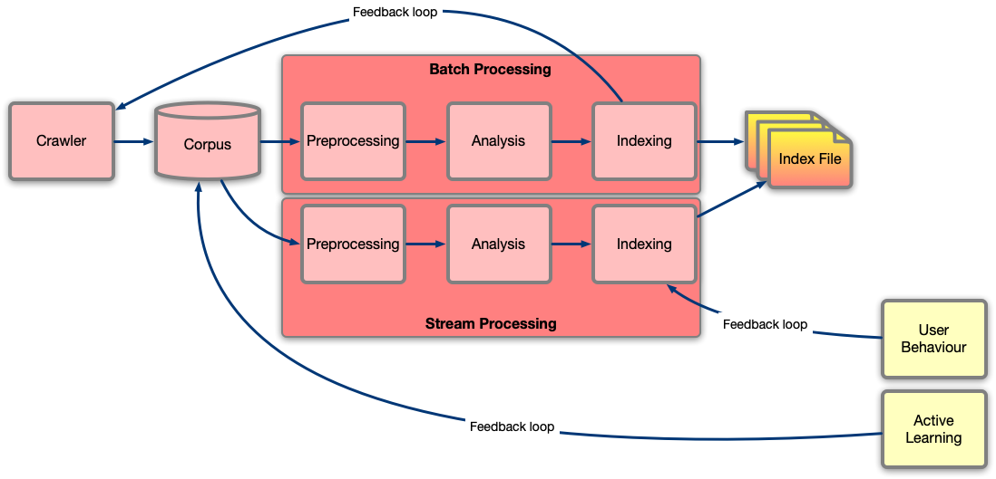
Given a corpus, the purpose of indexing is preprocessing, analysing and manipulating the documents and their metadata into data structures that optimise the retrieval phase. Most corpuses are very large, consisting of billions of documents, and require distributed indexing.
Preprocessing
The document is first preprocessed to bring it to a space with a consistent representation. For example, a document of research papers is brought to space of words, including title, abstract and body; then each word within the title, abstract and body is stemmed. Once all documents have been preprocessed, local variances disappear, and the corpus contains structured data. Similarly, in the case of images, EXIF data, size, compression, timestamp, location are extracted, and the image binary then treated as a an opaque byte array; the collection of these attributes is a document of structured data.
Analysis
The object of the analysis phase is to project the documents into a vector space where we can use some distance metric, e.g. euclidian, hamming, etc. to compare similarity between documents. For example, we can use characters as a consistent representation, and have a dictionary array {a, b, c, …} so that now we know the dimension 0 is a, 1 is b, and so forth. We can also use using linguistic analysis to work with a dictionary of words, phonemes, or fingerprints. The dictionary can also be a compressed version of word, for example the root morpheme, on top of which we can compare words by using the hamming distance metric. For document with opaque attributes, such as images, we can use computer vision, machine learning, AI, … to extract a vector representation. This could be a neural network output, as a vector mapping to a reduced set of labels (car, pedestrian, bus, road sign, work zone, …), or an internal vector representation of some intermediate layer within the network (embeddings).
Index Creation and Updates
Finally, the index creation pushes the results of the analysis into a physical data structure that can be used efficiently for retrieval. For example, if the result of our analysis is simply counting the number of times a word appears in a document, we could create an inverted index as a map of arrays, where the key of the map is a term, and the elements of the array are the documents where the term is found, starting with the document with most of occurrences of the word. In this case we could have [0, {(1,15), (5,9), (6,3)}], where the word referenced as the int 0 (for example “the”) is found in document-1 15 times, document-5 9 times, and document-6 3 times. Or perhaps,wWe could have also used TF-IDF (term-frequency / inverse-document-frequency), to calculate how many times the word “the” is found in the corpus in total, to promote the appearance of rare words in documents. There are many different possible indices, but the most interesting to us are the relational table, the inverted index, the vector database, and the neural network weights.
I bring up the neural network since for IR purposes it’s just one more possible data structure to describe a dataset of documents, but probabilistically. The index structure consists of the tensors of weights, and the search operation is the traversal of the network. Remember that the search query and the documents in the corpus need to brought back to the same space, i.e. Whatever we do to the search query, we do the same to the documents, so we can compare them. In the case of a NN, the weights capture the learnt state of the corpus, and putting a query through the document returns a vector, just like during training putting a document through the NN returns a vector in the same space.
With large corpuses, it’s likely that the index, or indices, will be very large, the size depending on which space we have chosen to project the documents into. This requires always sharding the index into fragments. One particularly important aspect is designing the physical index to allow incremental updates. For example, if our physical index on file for the inverted index would be as above [0, {(1,15), (5,9), (6,3)}], anytime we would find a new document with the word 0, we would need to update the whole array. By using a structure called posting lists, based on linked lists instead of arrays, we can become smarter about what to update and how to traverse the the docs during retrieval.
In practice, large inverted index databases, whether term based or vector based, are memory maps containing thousands of rows, which are computed and written to incrementally out-of-process, and then updated and loaded into memory as an atomic operation. With thousands of servers operating in a farm divided into shards and its replicas, memory maps allow high availability and high read throughput at low latency since the write-ops do not modify the index structures.
Preprocessing, analysis and indexing are long running computational jobs, whether in batch or in a streaming fashion, using technologies like Hadoop, Spark, BigTable/BigQuery to process them. Whereas in these offline systems we can have petabytes of data available and run complex analysis queries in order to create the index, the projection into the serving index produces a much smaller and leaner artefact exclusively optimised for a retrieval operation. This is why relational database are expensive for search, as the freedom they provide to find data in a variety of ways, introduces a significant storage and compute cost. Another side-effect is that whereas the total number of documents in a corpus could be trillions, the actual number of documents in the serving index may be millions or billions. For example, the web gets broken down into big lakes of documents, based on freshness and popularity.
Data Collection
The crawlers are responsible for collecting and storing documents that can later go into indexing. Other techniques could be scrapping for structured data, downloading full datasets, etc. Crawlers need to deal with priorities, scheduling, partial failures, rate limiting, etc. There is also a feedback loop from the indexing phase, to help not only know what to crawl, but also at what priority and frequency. This could apply to the web, but can also apply to cars in the road, knowing from which areas to upload, and at what priority and frequency, as well as managing upload budgets, in order not to deplete the crawler’s bandwidth allocation in popular things and miss rare events.
Crowdsourced User Behaviour Feedback Loops
A key innovation of web search in the late 1990s was having people help rank documents. This happened through two mechanisms:
- Inbound-outbound link counting
- Click-through-rate (CTR, click probability)
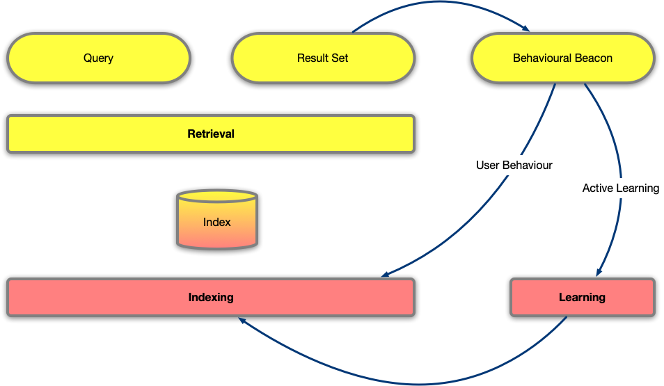
Particularly relevant for building Generative AI architectures is the feedback loop of CTR. With CTR, the system logs which results where shown the user, and which results are actually clicked on. By using this, we can calculate CTRs for results, and CTR maps for queries. Since the index contains probabilities, e.g. the TF-IDF weights, we can now adjust the prior probabilities with the observed behaviour (likelihood), in order to derive the posterior probabilities. As the system runs, it learns from user behaviour what is important. Behaviour does not simply end with clicks, but can also include bounce rate and dwell time.
A particular important part of the feedback loop is active learning. Although the most frequent use of active learning is the corpus analysis, to continuously improve models so that they better describe the corpus, active learning with manual or automated labelling (“expert”) can be used to analyse what does not get clicked on, but we thought should get clicked on. For example, in a neural network that learns and predicts (answers) aggregation queries, we may need to run SQL queries to further explain (obtain more/better samples) the expected output. If we expect the answer to a natural language query to be a natural language result, the SQL expert is automatically labelling the results which low likelihood. In the case of GenAI, we will see that this is a key component for how to design the system.
Practically speaking, the analysis of user behaviour results into a short term update of the index, and a long term one:
- Using an incremental distribution, such as GMP (Gamma-Poison), we can update the prior probabilities on the fly. In addition to reading the memory maps we talked about earlier, which contain the long-term prior probabilities, we read the short probability adjustments that allow us to calculate on the fly posterior probabilities using the observed user likelihood.
- Capturing user behaviour during the index creation, so that the next time we create the memory map, it already includes learnt click behaviour, and benefits from the expert annotation.
Summary Learnings Applicable to Generative AI
As we have now walked through the flow of search, we can call out the main things that are relevant to GenAI:
- IR systems are the composition of a number of backend search applications.
- A key ingredient is mapping queries (questions) to which backends to use, and how.
- A backend is an inverted index, a vector database or a model of weights, all of them capturing a distribution of priors as a physical index, which can and must be sharded.
- Feedback loops from crowdsourced user behaviour are critical to continuously improve our analysis of the dataset, but also the ranking.